|
New in Excel 2010 is the AGGREGATE Function. Have you ever had the need to redo a calculation because the total you had sums an entire column whereas suddenly, you realize you have to hide some rows? In the screenshot below, you can immediately see that the items should not total at 14000. Upon further checking, you may see that some rows were hidden, and the formula =SUM(E2:E15) adds all cells in the range, including those hidden rows. 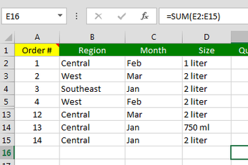 With the AGGREGATE function, the cell with the total will update based on what is only visible in the worksheet. The function uses codes to be created. When you enter the open parenthesis after the function, Excel will show a dropdown list where you could choose the code number for your desired operation. Since we want to add numbers, we choose 9. =AGGREGATE(9, ... 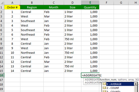 The next argument the function needs is what to ignore. Here you can see that AGGREGATE also allows you to ignore error cells. This is a way to resolve doing an AVERAGE but one of the cells in the range is an error (which means you will get an error too when you do an AVERAGE.) Since we need to ignore hidden rows, we choose 5 in the option and type it in the formula. =AGGREGATE(9,5 ... 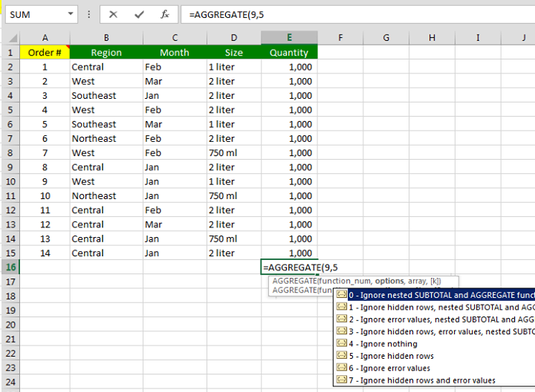 Finally, add the range as the third argument. =AGGREGATE(9,5,E2:E15) The formula now updates based on what is only visible in the worksheet. 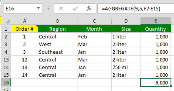 |

Archives
April 2020
Categories |
Menu

 RSS Feed