|
1. TEXTJOIN This function is an evolution of the old CONCATENATE function. TEXTJOIN allows concatenation of an entire range with a specified delimiter. To combine the column data into a full address, the formula would be: =TEXTJOIN(", ",1,A2:D2) •The first argument is the delimiter. This is what will separate the values. •The second argument is either TRUE or FALSE. Indicating this as TRUE or 1 means it will ignore empty cells. As FALSE, it would consider empty cells and still show them in the result. 2. CONCAT CONCAT is obviously another evolution of CONCATENATE. Using the previous example, if CONCAT is used, it will result to: CONCAT only accepts one kind of argument, which is the range. It will combine the texts, that’s all. No delimiter can be set, nor ability to ignore blanks. Therefore, it is a more basic kind of TEXTJOIN. =CONCAT(A2:D2) Similar to TEXTJOIN, the #VALUE error will show up if the result is more than 32767 characters. 3. IFS The IFS function has been introduced to handle a situation where you will string several IF statements in one. =IFS (B2<=80,"Fail" , B2<=90,"Good" , B2>90,"Pass" ) Note that unlike in the nested IF, the IFS function does not allow a “catch rest” or the last argument in a multiple IFs formula. All possible outcomes must have their corresponding logical test. 4. SWITCH The SWITCH is similar to the old CHOOSE function, but is not limited in accepting numbers in order. It is used to simply conditional statements. =SWITCH( A2 , "Japan","Asia" , "France","Europe" , "Philippines","Asia" )
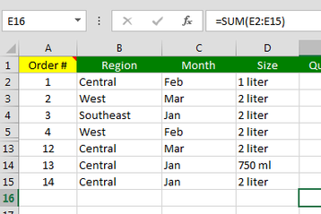
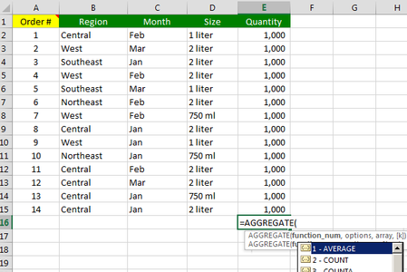
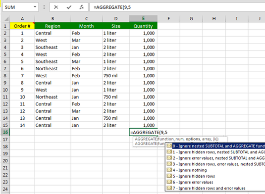
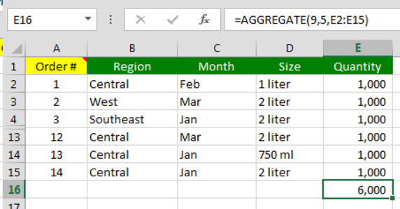
The formula starts with cell to be evaluated. Then succeeding values and their corresponding outcomes follow. In the example, if A2 is “Japan,” then the result will be “Asia.” If A2 is “France,” the result is “Europe.” New in Excel 2010 is the AGGREGATE Function. Have you ever had the need to redo a calculation because the total you had sums an entire column whereas suddenly, you realize you have to hide some rows? In the screenshot below, you can immediately see that the items should not total at 14000. Upon further checking, you may see that some rows were hidden, and the formula =SUM(E2:E15) adds all cells in the range, including those hidden rows. With the AGGREGATE function, the cell with the total will update based on what is only visible in the worksheet. The function uses codes to be created. When you enter the open parenthesis after the function, Excel will show a dropdown list where you could choose the code number for your desired operation. Since we want to add numbers, we choose 9. =AGGREGATE(9, ... The next argument the function needs is what to ignore. Here you can see that AGGREGATE also allows you to ignore error cells. This is a way to resolve doing an AVERAGE but one of the cells in the range is an error (which means you will get an error too when you do an AVERAGE.) Since we need to ignore hidden rows, we choose 5 in the option and type it in the formula. =AGGREGATE(9,5 ... Finally, add the range as the third argument. =AGGREGATE(9,5,E2:E15)
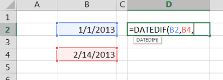
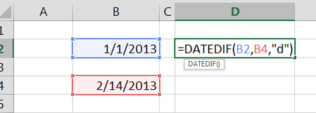
The formula now updates based on what is only visible in the worksheet. "DATEDIF" is one of the "phased out" functions in Excel but it still there if you need it. However, it is not documented in Excel and when you start the function, it does not show its elements so you really need to know how to use it because Excel won't guide you. DATEDIF determines the difference between two dates. This has been replaced by advanced and more flexible functions DAYS, NETWORKDAYS, and WORKDAYS, together with their .INTL counterparts but DATEDIF still can be handy. The funtions works: =DATEDIF(startdate, enddate, intervaltype) The interval type is a code to determine what you are counting between the dates. You can hardcode the constant letters in between quotation marks (") as the third element in the function. This will show 44 because we used letter "d" and there are 44 complete days between Jan 1 2013 and Feb 1 2013. I have to emphasize "complete" because if you are using other time intervals, it will give you the number of complete months, years, etc. Other codes that can be used:
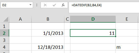
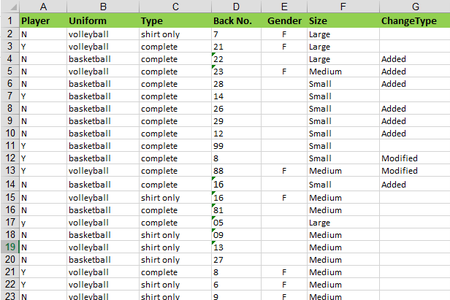
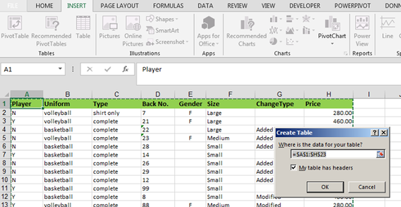
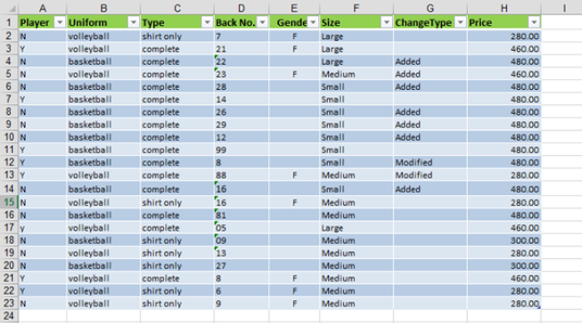
"m" for months "y" for years "d" for days then the "combo": "ym" which counts the complete calendar months as if they were on the same year (so Jan 1 2013 and Feb 1 2014 will be just 1 unlike if you use "m" which will you 13,) "yd" which counts the complete calendar days as if they were on the same year, and "md" which counts the complete calendar days as if they were on the same month and year. You can also use other cells to give you the interval types which can come handy if you are playing with the function. [Excel 2007 onwards] If you create a data like below, and ask someone if this is a table, 95% would say it is. But in Excel's world, this is just a range. A range is any data setup either in row, column, or table- like. A table or data table in Excel is defined differently and has to be declared. To create a table, you need to setup something like the table or a range. Once done, we need to declare that this range of cells is a table by going to Insert > Table. (This is available in 2003, under the Data dropdown.) A small window will appear and you can enter the range of cells that will be declared a table. If you have selected one cell of the range or the entire range, then, this should be filled out automatically. Click OK and your data range will transform to a data table, which is shown by default to have horizontal bars and drop downs if it does not have yet. Note that it will not override any previous cell formatting you may have added. You can change the formattings of your data table by clicking any cell and going to the Table Tools > Design tab, a context ribbon that will show up.
One nice feature of the data table is that when it is a large one and you have to scroll, you do not have to freeze the panes to maintain visibility of the headers. When you were declaring the range as a table, and you checked the box that says "My Table has Headers," the first row of the table will be the headers, and they will replace the letters of the heading (the A, B, C, D, etc above the worksheet) when you scroll down. More features of the data table will be explored in the next entries. |
Archives
April 2020
Categories |





 RSS Feed